介绍
DNA Methylation和疾病的发生发展存在密切相关,它一般通过CH3替换碱基5‘碳的H原子,进而调控基因的转录。常用的DNA methylation是Illumina Infinium methylation arrays,该芯片有450K和850K(也即是EPIC)。
该脚本基于命令行模式运行:主要分为以下几部分
-
读取IDAT(甲基化芯片数据格式)数据和建立RGset对象;
-
质控(根据QC结果质控和根据强度P值小于0.01或0.05过滤);
-
标准化
-
过滤:
-
检测P值过滤;
-
去重复;
-
去除X和Y染色体的甲基化;
-
去除CpG岛的SNPs;
-
去除多比对的甲基化
- 输出matrix
准备文件
- Sample.csv: csv格式的table

- DNA methylation folder
IDAT/
├── 202250800017
│   ├── 202250800017_R01C01_Grn.idat
│   ├── 202250800017_R01C01_Red.idat
│   ├── 202250800017_R02C01_Grn.idat
│   ├── 202250800017_R02C01_Red.idat
│   ├── 202250800017_R03C01_Grn.idat
│   ├── 202250800017_R03C01_Red.idat
│   ├── 202250800017_R04C01_Grn.idat
│   ├── 202250800017_R04C01_Red.idat
│   ├── 202250800017_R05C01_Grn.idat
│   ├── 202250800017_R05C01_Red.idat
│   ├── 202250800017_R06C01_Grn.idat
│   ├── 202250800017_R06C01_Red.idat
│   ├── 202250800017_R07C01_Grn.idat
│   ├── 202250800017_R07C01_Red.idat
│   ├── 202250800017_R08C01_Grn.idat
│   └──202250800017_R08C01_Red.idat
├── 202250800184
│   ├── 202250800184_R01C01_Grn.idat
│   ├── 202250800184_R01C01_Red.idat
│   ├── 202250800184_R02C01_Grn.idat
│   ├── 202250800184_R02C01_Red.idat
│   ├── 202250800184_R03C01_Grn.idat
│   ├── 202250800184_R03C01_Red.idat
│   ├── 202250800184_R04C01_Grn.idat
│   ├── 202250800184_R04C01_Red.idat
│   ├── 202250800184_R05C01_Grn.idat
│   ├── 202250800184_R05C01_Red.idat
│   ├── 202250800184_R06C01_Grn.idat
│   ├── 202250800184_R06C01_Red.idat
│   ├── 202250800184_R07C01_Grn.idat
│   ├── 202250800184_R07C01_Red.idat
│   ├── 202250800184_R08C01_Grn.idat
│   └── 202250800184_R08C01_Red.idat
- cross reactive probes files
850K: 13059_2016_1066_MOESM1_ESM_cross-reactive_probes.csv
450K: 48639-non-specific-probes-Illumina450k.csv
loading R packages
library(dplyr)
library(limma)
library(minfi)
library(missMethyl)
library(minfiData)
library(stringr)
library(ENmix)
library(RColorBrewer)
library(optparse)
get options
option_list = list(
  make_option(c("-f", "--folder"), type="character", default=".",
        help="folder with idat files [default= %default]", metavar="character"),
  make_option(c("-t", "--target"), type="character", default=".",
        help="target file with sample information [default= %default]", metavar="character"),
  make_option(c("-a", "--array"), type="character", default=".",
        help="the type of DNA chip array file [default= %default]", metavar="character"),
  make_option(c("-o", "--out"), type="character", default="out",
        help="output directory name [default= %default]", metavar="character")
);
opt_parser <- OptionParser(option_list=option_list);
opt <- parse_args(opt_parser);
print(opt)
Creating output directory
create_dir <- function(dirpath){

  if(!dir.exists(dirpath)){
    dir.create(dirpath, recursive = TRUE)
  }
}
# current dir
current_dir <- getwd()
# Result & QC dir
out_dir <- opt$out
qc_dir <- paste0(out_dir, "/QC")
create_dir(qc_dir)
# DataSet dir
set_dir <- paste0(out_dir, "/Set")
create_dir(set_dir)
# Matrix dir
raw_dir <- paste0(out_dir, "/Matrix")
create_dir(raw_dir)
Chip Array annotation and cross reactive files
if(opt$chip == "850k"){
  # For HumanMethylationEPIC bead chip array files (850k) load the following two packages and two files
  library(IlluminaHumanMethylationEPICmanifest)
  library(IlluminaHumanMethylationEPICanno.ilm10b4.hg19)
  ann <- getAnnotation(IlluminaHumanMethylationEPICanno.ilm10b4.hg19)
  crossreac_probes <- read.csv("/disk/user/zouhua/pipeline/methylseq_IDAT/util/13059_2016_1066_MOESM1_ESM_cross-reactive_probes.csv")
}else if(opt$chip == "450k"){
  # For HumanMethylation450 bead chip array files (450k) load the following packages and two files
  library(IlluminaHumanMethylation450kmanifest)
  library(IlluminaHumanMethylation450kanno.ilmn12.hg19)
  ann <- getAnnotation(IlluminaHumanMethylation450kanno.ilmn12.hg19)
  crossreac_probes <- read.csv("/disk/user/zouhua/pipeline/methylseq_IDAT/util/48639-non-specific-probes-Illumina450k.csv")
}
Reading idat files
# list the files
list.files(opt$folder, recursive = TRUE)
# read in the sample sheet for the experiment
targets <- read.csv(opt$target)
head(targets)
Creating RGset files
RGSet <- read.metharray.exp(targets = targets)
targets$ID <- paste(targets$Sample_Name)
sampleNames(RGSet) <- targets$ID
print(RGSet)
Quality Checks
# C.1. Plot quality control plots (package ENmix)
setwd(qc_dir)
plotCtrl(RGSet)

# C.2. Make PDF QC report (package minfi)
# To include colouring samples by variable such as sentrix position include argument: sampGroups=targets$sentrix_pos
setwd(current_dir)
qcReport_pdf <- paste0(qc_dir, "/qcReport.pdf")
qcReport(RGSet, sampNames = targets$Sample_Name, pdf = qcReport_pdf)

# C.3. Make pre-normalisation beta density plots
# Here samples are coloured by sentrix position
nb.levels <- length(unique(targets$Array))
mycolors <- colorRampPalette(brewer.pal(8, "Dark2"))(nb.levels)
jpeg(paste0(qc_dir, "/UnormalisedBetaDensityPlot_bySentrixPosition.jpg"), width = 800, height = 800)
densityPlot(RGSet, sampGroups = targets$Array, pal = mycolors, ylim = c(0, 5))
dev.off()

# C.4. Create MethylSet, RatioSet, then a GenomicRatioSet for further QC
MSet <- preprocessRaw(RGSet)
ratioSet <- ratioConvert(MSet, what = "both", keepCN = TRUE)
gset <- mapToGenome(ratioSet, mergeManifest = T)

# C.5. Perform QC on MSet and plot methylated versus unmethylated intensities
qc <- getQC(MSet)
pdf(paste0(qc_dir, "/Meth-unmeth_intensities.pdf"), height = 4, width = 4)
par(mfrow = c(1, 1), family = "Times", las = 1)
plotQC(qc) # If U and/or M intensity log medians are <10.5, sample is by default of bad quality
dev.off()

# C.6. remove any samples with meth or unmeth intensity < 10.5, then remove from all previous files
if(sum(rowMeans(as.data.frame(qc)) < 10.5 ) > 0) {
  print(paste("Warning: sample", rownames(qc)[rowMeans(as.data.frame(qc)) < 10.5],
              "has mean meth-unmeth signal intensity <10.5. Remove sample."))
}
keep.samples <- apply(as.data.frame(qc), 1, mean) > 10.5
RGSet_remain <- RGSet[, keep.samples]
MSet_remain <- MSet[, keep.samples]
ratioSet_remain <- ratioSet[, keep.samples]
gset_remain <- gset[, keep.samples]
targets_remain <- targets[keep.samples, ]

###############################################################
########    Calculate detection p values and plot      ########
###############################################################
# Here the samples are coloured by sentrix ID to check for poor performing chips
detP <- detectionP(RGSet_remain)
pdf(paste0(qc_dir, "/detection_pvalues.pdf"), height = 4, width = 4)
par(mfrow = c(1, 1), family = "Times", las = 1)
barplot(colMeans(detP),
        col = as.numeric(factor(targets$Slide)),
        las = 2,
        cex.names = 0.8,
        ylim = c(0, 0.05),
        ylab = "Mean detection p-values")
abline(h = 0.01 ,col = "red")
dev.off()

if(sum(colMeans(detP) > 0.01) > 0){
  print(paste("Warning: sample", names(colMeans(detP))[colMeans(detP) > 0.01],
              "has >0.01 mean detection p-value. Remove sample"))
}
# If required: remove any samples with detection p value > 0.01, then remove from all previous files
keep.samples_v2 <- apply(detP, 2, mean) < 0.01
RGSet_remain_v2 <- RGSet_remain[, keep.samples_v2]
MSet_remain_v2 <- MSet_remain[, keep.samples_v2]
ratioSet_remain_v2 <- ratioSet_remain[, keep.samples_v2]
gset_remain_v2 <- gset_remain[, keep.samples_v2]
targets_remain_v2 <- targets_remain[keep.samples_v2, ]
glimpse(targets_remain_v2)
output raw set files
save(RGSet, file = paste0(set_dir, "/RGSet_Raw.RData"))
save(MSet, file = paste0(set_dir, "/MSet_Raw.RData"))
save(gset, file = paste0(set_dir, "/gset_Raw.RData"))

save(RGSet_remain, file = paste0(set_dir, "/RGSet_trim_intensity.RData"))
save(MSet_remain, file = paste0(set_dir, "/MSet_trim_intensity.RData"))
save(gset_remain, file = paste0(set_dir, "/gset_trim_intensity.RData"))

save(RGSet_remain_v2, file = paste0(set_dir, "/RGSet_trim_detection.RData"))
save(MSet_remain_v2, file = paste0(set_dir, "/MSet_trim_detection.RData"))
save(gset_remain_v2, file = paste0(set_dir, "/gset_trim_detection.RData"))

size.RGSet_remain_v2 <- as.data.frame(t(dim(RGSet_remain_v2)))
size.MSet_remain_v2 <- as.data.frame(t(dim(MSet_remain_v2)))
size.gset_remain_v2 <- as.data.frame(t(dim(gset_remain_v2)))
Create raw unormalised and unfiltered beta table for later comparison
betaRaw <- getBeta(gset_remain_v2)
mRaw <- getM(gset_remain_v2)

save(betaRaw, file = paste0(raw_dir, "/betaRaw.RData"))
save(mRaw, file = paste0(raw_dir, "/mRaw.RData"))
Normalization
RGSet_norm <- preprocessFunnorm(RGSet_remain_v2)
size.RGSet_norm <- as.data.frame(t(dim(RGSet_norm)))
save(RGSet_norm, file = paste0(set_dir, "/RGSet_normalization.RData"))

# visualise what the data looks like before and after normalisation
pdf(paste0(raw_dir, "/normalisation_status.pdf"), height = 4, width = 4)
par(mfrow=c(1,2))
densityPlot(RGSet_remain_v2, sampGroups=targets$Sample_Source, main="Raw", legend=FALSE)
legend("top", legend = levels(factor(targets$Sample_Source)),
       text.col=brewer.pal(8,"Dark2"))
densityPlot(getBeta(RGSet_norm), sampGroups=targets$Sample_Source,
            main="Normalized", legend=FALSE)
legend("top", legend = levels(factor(targets$Sample_Source)),
       text.col=brewer.pal(8, "Dark2"))
dev.off()
Data exploration
# MDS plots to look at largest sources of variation
pal <- brewer.pal(8,"Dark2")
pdf(paste0(raw_dir, "/Data_exploration_PCA.pdf"), height = 4, width = 4)
par(mfrow=c(1, 2))
plotMDS(getM(RGSet_norm), top=1000, gene.selection="common",
        col=pal[factor(targets$Sample_Group)])
legend("top", legend=levels(factor(targets$Sample_Group)), text.col=pal,
       bg="white", cex=0.7)
plotMDS(getM(RGSet_norm), top=1000, gene.selection="common",
        col=pal[factor(targets$Sample_Source)])
legend("top", legend=levels(factor(targets$Sample_Source)), text.col=pal,
       bg="white", cex=0.7)
dev.off()

# Examine higher dimensions to look at other sources of variation
pdf(paste0(raw_dir, "/Data_exploration_PCA_v2.pdf"), height = 4, width = 6)
par(mfrow=c(1, 3))
plotMDS(getM(RGSet_norm), top=1000, gene.selection="common",
        col=pal[factor(targets$Sample_Group)], dim=c(1,3))
legend("top", legend=levels(factor(targets$Sample_Group)), text.col=pal,
       cex=0.7, bg="white")

plotMDS(getM(RGSet_norm), top=1000, gene.selection="common",
        col=pal[factor(targets$Sample_Group)], dim=c(2,3))
legend("topleft", legend=levels(factor(targets$Sample_Group)), text.col=pal,
       cex=0.7, bg="white")

plotMDS(getM(RGSet_norm), top=1000, gene.selection="common",
        col=pal[factor(targets$Sample_Group)], dim=c(3,4))
legend("topright", legend=levels(factor(targets$Sample_Group)), text.col=pal,
       cex=0.7, bg="white")
dev.off()
filtering
# ensure probes are in the same order in the mSetSq and detP objects
detP <- detP[match(featureNames(RGSet_norm), rownames(detP)), ]

# remove any probes that have failed in one or more samples
keep <- rowSums(detP < 0.01) == ncol(RGSet_norm)
table(keep)
RGSet_normFlt <- RGSet_norm[keep, ]
RGSet_normFlt

# removing duplicated
pData <- pData(RGSet_normFlt)
pData2 <- pData[order(pData(RGSet_normFlt)$Sample_Name), ]
dim(pData2)
head(pData2)

dups <- pData2$Sample_Name[duplicated(pData2$Sample_Name)]
if( length(dups) > 0 ){
    whdups     <- lapply(dups, function(x){which(pData2$Sample_Name == x)})
    whdups2rem <- sapply(1:length(dups), function(i) rbinom(1, 1, prob = 1/length(whdups[[1]])))+1
    torem <- sapply(1:length(whdups), function(i){whdups[[i]][whdups2rem[i]]})
    pData2 <- pData2[-torem, ]
}
RGSet_norm_duplicate <- RGSet_normFlt[, rownames(pData2)]
save(RGSet_norm_duplicate, file = paste0(set_dir, "/RGSet_norm_duplicate.RData"))
size.detP <- as.data.frame(t(dim(RGSet_norm_duplicate)))

# if your data includes males and females, remove probes on the sex chromosomes
keep <- !(featureNames(RGSet_norm_duplicate) %in% ann$Name[ann$chr %in%
                                                        c("chrX","chrY")])
table(keep)
RGSet_norm_duplicate <- RGSet_norm_duplicate[keep, ]

# remove probes with SNPs at CpG site
RGSetFlt <- dropLociWithSnps(RGSet_norm_duplicate)
RGSetFlt

# exclude cross reactive probes
keep <- !(featureNames(RGSetFlt) %in% crossreac_probes$TargetID)
table(keep)
RGSetFlt <- RGSetFlt[keep,]
RGSetFlt

pdf(paste0(raw_dir, "/filtered_status.pdf"), height = 4, width = 4)
par(mfrow=c(1, 2))
plotMDS(getM(RGSet_norm), top=1000, gene.selection="common", main="Normalized",
        col=pal[factor(targets$Sample_Source)])
legend("top", legend=levels(factor(targets$Sample_Source)), text.col=pal,
       bg="white", cex=0.7)
plotMDS(getM(RGSetFlt), top=1000, gene.selection="common", main="Normalized_filter",
        col=pal[factor(targets$Sample_Source)])
legend("top", legend=levels(factor(targets$Sample_Source)), text.col=pal,
       bg="white", cex=0.7)
dev.off()
Normalization matrix
betaNorm <- getBeta(RGSetFlt)
dim(betaNorm)
size.betaNorm <- as.data.frame(t(dim(betaNorm)))

mNorm <- getM(RGSetFlt)
dim(mNorm)
size.mNorm <- as.data.frame(t(dim(mNorm)))

# visualization
pdf(paste0(raw_dir, "/filtered_status.pdf"), height = 4, width = 4)
par(mfrow=c(1,2))
densityPlot(betaNorm, sampGroups=targets$Sample_Group, main="Beta values",
            legend=FALSE, xlab="Beta values")
legend("top", legend = levels(factor(targets$Sample_Group)),
       text.col=brewer.pal(8,"Dark2"))
densityPlot(mNorm, sampGroups=targets$Sample_Group, main="M-values",
            legend=FALSE, xlab="M values")
legend("topleft", legend = levels(factor(targets$Sample_Group)),
       text.col=brewer.pal(8,"Dark2"))
dev.off()

# Check for NA and -Inf values
betaRaw.na <- betaRaw[!complete.cases(betaRaw), ]
dim(betaRaw.na)
NAbetas <- rownames(betaRaw.na)
betaNAsNorm <- betaNorm[rownames(betaNorm) %in% NAbetas, ] # Should be [1] 0 x ncol(betaNorm)

# Check for infinite values in m table, replace in the no infinite values m table
TestInf <- which(apply(mNorm, 1, function(i)sum(is.infinite(i))) > 0)
save(TestInf, file = paste0(set_dir, "/InfiniteValueProbes.RData"))
mNoInf <- mNorm
mNoInf[!is.finite(mNoInf)] <- min(mNoInf[is.finite(mNoInf)])
TestInf2 <- which(apply(mNoInf, 1, function(i) sum(is.infinite(i))) > 0)
TestInf2 # Should be named integer(0)
size.mNoInf <- as.data.frame(t(dim(mNoInf)))

# Write tables
write.table(targets_remain_v2, file=paste0(raw_dir, "/TargetsFile.csv"), sep=",", col.names=NA)
write.table(betaNorm, file=paste0(raw_dir, "/NormalisedFilteredBetaTable.csv"), sep=",", col.names=NA)
write.table(mNorm, file=paste0(raw_dir, "/NormalisedFilteredMTable.csv"), sep=",", col.names=NA)
write.table(mNoInf, file=paste0(raw_dir, "/NormalisedFilteredMTable_noInf.csv"), sep=",", col.names=NA)
Create dimensions table
DimensionsTable <- rbind(size.RGSet_remain_v2, size.MSet_remain_v2, size.gset_remain_v2,
                         size.RGSet_norm, size.detP,
                         size.betaNorm, size.mNorm, size.mNoInf)
rownames(DimensionsTable) <- c("RGset_size", "MSet_size", "gset_size",
                               "fun_size", "detP_lost",
                               "beta_size", "m_size", "mNoInf_size")
colnames(DimensionsTable) <- c("Probe_number", "Sample_number")
write.table(DimensionsTable, file=paste0(out_dir, "/DimensionsTable.txt"), sep="\t", col.names=NA)
运行
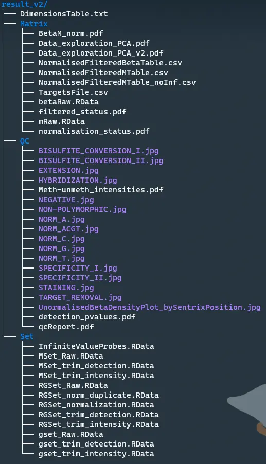
Rscript DNA_Methylation.R -f IDAT -t Sample.csv -a 850k -o result_v2
Software versions
sessionInfo()
R version 4.0.2 (2020-06-22)
Platform: x86_64-conda_cos6-linux-gnu (64-bit)
Running under: CentOS Linux 8 (Core)

Matrix products: default
BLAS/LAPACK: /disk/share/anaconda3/lib/libopenblasp-r0.3.10.so

locale:
 [1] LC_CTYPE=en_US.UTF-8       LC_NUMERIC=C               LC_TIME=en_US.UTF-8
 [4] LC_COLLATE=en_US.UTF-8     LC_MONETARY=en_US.UTF-8    LC_MESSAGES=en_US.UTF-8
 [7] LC_PAPER=en_US.UTF-8       LC_NAME=C                  LC_ADDRESS=C
[10] LC_TELEPHONE=C             LC_MEASUREMENT=en_US.UTF-8 LC_IDENTIFICATION=C

attached base packages:
[1] stats4    parallel  stats     graphics  grDevices utils     datasets  methods   base

other attached packages:
 [1] RColorBrewer_1.1-2                                  ENmix_1.26.9
 [3] doParallel_1.0.16                                   stringr_1.4.0
 [5] minfiData_0.36.0                                    IlluminaHumanMethylation450kmanifest_0.4.0
 [7] missMethyl_1.24.0                                   IlluminaHumanMethylationEPICanno.ilm10b4.hg19_0.6.0
 [9] IlluminaHumanMethylation450kanno.ilmn12.hg19_0.6.0  minfi_1.36.0
[11] bumphunter_1.32.0                                   locfit_1.5-9.4
[13] iterators_1.0.13                                    foreach_1.5.1
[15] Biostrings_2.58.0                                   XVector_0.30.0
[17] SummarizedExperiment_1.20.0                         Biobase_2.50.0
[19] MatrixGenerics_1.2.1                                matrixStats_0.58.0
[21] GenomicRanges_1.42.0                                GenomeInfoDb_1.26.4
[23] IRanges_2.24.1                                      S4Vectors_0.28.1
[25] BiocGenerics_0.36.0                                 limma_3.46.0
[27] dplyr_1.0.5

loaded via a namespace (and not attached):
  [1] AnnotationHub_2.22.0          BiocFileCache_1.14.0          plyr_1.8.6
  [4] splines_4.0.2                 BiocParallel_1.24.1           digest_0.6.27
  [7] htmltools_0.5.1.1             RPMM_1.25                     fansi_0.4.2
 [10] magrittr_2.0.1                memoise_2.0.0                 cluster_2.1.0
 [13] readr_1.4.0                   annotate_1.68.0               askpass_1.1
 [16] siggenes_1.64.0               lpSolve_5.6.15                prettyunits_1.1.1
 [19] blob_1.2.1                    rappdirs_0.3.3                xfun_0.20
 [22] crayon_1.4.1                  RCurl_1.98-1.3                jsonlite_1.7.2
 [25] genefilter_1.72.0             GEOquery_2.58.0               impute_1.64.0
 [28] survival_3.2-10               glue_1.4.2                    zlibbioc_1.36.0
 [31] DelayedArray_0.16.3           irr_0.84.1                    Rhdf5lib_1.12.1
 [34] HDF5Array_1.18.1              DBI_1.1.1                     rngtools_1.5
 [37] Rcpp_1.0.6                    xtable_1.8-4                  progress_1.2.2
 [40] bit_4.0.4                     mclust_5.4.7                  preprocessCore_1.52.1
 [43] httr_1.4.2                    gplots_3.1.1                  ellipsis_0.3.1
 [46] pkgconfig_2.0.3               reshape_0.8.8                 XML_3.99-0.6
 [49] sass_0.3.1                    dbplyr_2.1.1                  utf8_1.2.1
 [52] dynamicTreeCut_1.63-1         later_1.1.0.1                 tidyselect_1.1.0
 [55] rlang_0.4.10                  AnnotationDbi_1.52.0          BiocVersion_3.12.0
 [58] tools_4.0.2                   cachem_1.0.4                  generics_0.1.0
 [61] RSQLite_2.2.5                 ExperimentHub_1.16.0          evaluate_0.14
 [64] fastmap_1.1.0                 yaml_2.2.1                    org.Hs.eg.db_3.12.0
 [67] knitr_1.31                    bit64_4.0.5                   beanplot_1.2
 [70] caTools_1.18.2                scrime_1.3.5                  purrr_0.3.4
 [73] nlme_3.1-150                  doRNG_1.8.2                   sparseMatrixStats_1.2.1
 [76] mime_0.10                     nor1mix_1.3-0                 xml2_1.3.2
 [79] biomaRt_2.46.3                compiler_4.0.2                rstudioapi_0.13
 [82] interactiveDisplayBase_1.28.0 curl_4.3                      tibble_3.1.0
 [85] statmod_1.4.35                geneplotter_1.66.0            bslib_0.2.4
 [88] stringi_1.4.6                 GenomicFeatures_1.42.2        lattice_0.20-41
 [91] Matrix_1.3-2                  multtest_2.46.0               vctrs_0.3.7
 [94] pillar_1.6.0                  lifecycle_1.0.0               rhdf5filters_1.2.0
 [97] BiocManager_1.30.12           jquerylib_0.1.3               data.table_1.14.0
[100] bitops_1.0-6                  httpuv_1.5.5                  rtracklayer_1.50.0
[103] R6_2.5.0                      promises_1.2.0.1              KernSmooth_2.23-18
[106] codetools_0.2-18              gtools_3.8.2                  MASS_7.3-53.1
[109] assertthat_0.2.1              rhdf5_2.34.0                  openssl_1.4.3
[112] GenomicAlignments_1.26.0      Rsamtools_2.6.0               GenomeInfoDbData_1.2.4
[115] hms_1.0.0                     quadprog_1.5-8                grid_4.0.2
[118] tidyr_1.1.3                   base64_2.0                    rmarkdown_2.7
[121] DelayedMatrixStats_1.12.3     illuminaio_0.32.0             shiny_1.6.0
[124] tinytex_0.31
参考
-
minfi tutorial
-
The Chip Analysis Methylation Pipeline
-
A cross-package Bioconductor workflow for analysing methylation array data
-
Methylation_analysis_scripts